Connections and interpretations

Inverse reinforcement learning
- we have the expert policy (inferred from the gold standard in the training data)
- we infer the per-action reward function (rollin/out)
LOLS with classifier only rollouts is RL (Chang et al., 2015)
Bandit learning
Rolling out each action can be expensive:
- many possible actions
- expensive loss functions to calculate
What if we only rollout one?
Bandit Learning
Structured Contextual Bandit LOLS (Chang et al., 2015)
Sokolov et al. (2016) used bandit feedback for chunking
Semi/Unsupervised learning
Learning with non-decomposable loss functions means
- no need to know the correct actions
- learn to predict them in order to minimize the loss
UNSEARN (Daumé III, 2009): Predict the structured output so that you can predict the input from it (auto-encoder!)
Negative data sampling
paths = [[],[(0,4),(1,3)],[(0,4),(1,3),(2,2)],[(0,4),(1,3),(2,2),(3,1)]]
rows = ['Noun', 'Verb', 'Modal', 'Pronoun','NULL']
columns = ['NULL','I', 'can', 'fly']
gold_path = [(0,4),(1,3),(2,2),(3,1)]
cbs=[]
cb_gold = cg.draw_cost_breakdown(rows, columns, gold_path)
cbs.append(cb_gold)
wrong_path = [(0,4),(1,2)]
cb_wrong = cg.draw_cost_breakdown(rows, columns, wrong_path)
cbs.append(cb_wrong)
p = gold_path.copy()
for i in range(4):
    p = gold_path.copy()
    p[2] = (gold_path[2][0],i)
    if p == gold_path:
        cost = 0
    elif i==1:
        cost =2
        p[3] = (3,0)
    else:
        cost = 1
    cbs.append(cg.draw_cost_breakdown(rows, columns, p, cost, p[3], roll_in_cell=p[1],roll_out_cell=(3,0), explore_cell=p[2]))
util.Carousel(cbs)
- Expert action sequence → positive example
- All other action sequences → negative examples
Generate useful negative samples around the expert, related to adversarial training (Ho and Ermon, 2016) )
Coaching
If the optimal action is difficult to
predict, the coach teaches a good one
that is easier (He et al., 2012)

Expert: $\alpha^{\star}= \mathop{\arg \min}_{\alpha \in {\cal A}} L(S_t(\alpha,\pi^{\star}),\mathbf{y})$
Coach: $\alpha^{\dagger}= \mathop{\arg \min}_{\alpha \in {\cal A}} \lbrace L(S_t(\alpha,\pi^{\star}),\mathbf{y}) - \lambda \cdot f(\alpha, \mathbf{x}, S_t)\rbrace$
i.e. $\alpha^{\dagger}=\mathop{\arg \min}_{\alpha \in {\cal A}} \lbrace loss(\alpha) - \lambda \cdot classifier(\alpha) \rbrace$
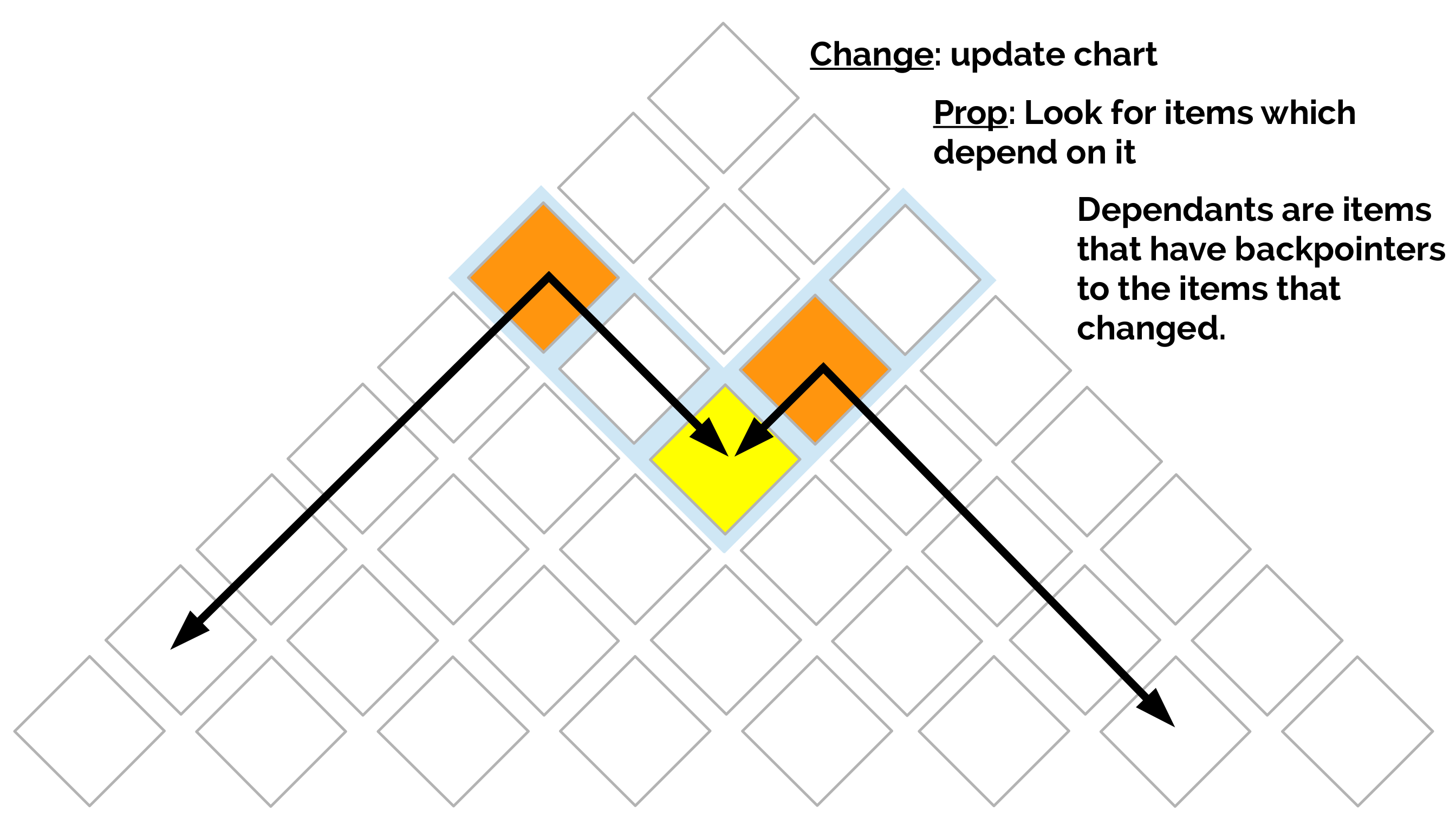
Changeprop
Speed-up action costing in LOLS (Viera and Eisner, 2016):
If one action changes, don't assess the cost of the whole trajectory (under assumptions), propagate the change!
 </a>
</a>
What about Recurrent Neural Networks?
They face similar problems:
- trained at the word rather than sentence level
- assume previous predictions are correct
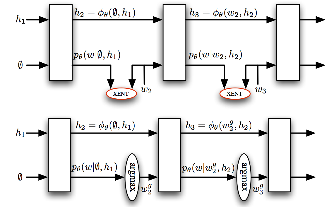
Imitation learning and RNNs
- DAgger mixed rollins, similar to scheduled sampling (Bengio et al., 2015)
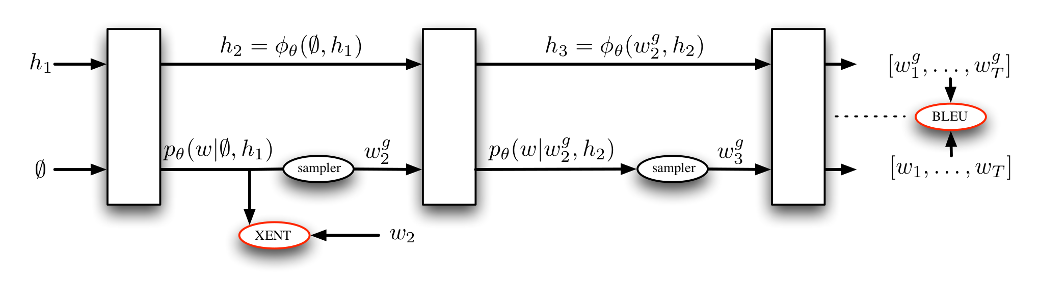
- MIXER (Ranzato et al., 2016): Mix REINFORCE-ment learning with imitation: we have the expert policy!
- no rollouts, learn a regressor to estimate action costs
- end-to-end back propagation through the sequence
Actor-critic
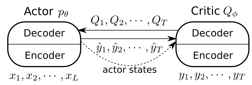
- actor: the RNN we are learning to use during testing
- critic: another RNN that is trained to predict the value of the actions of the critic
Summary so far
- basic concepts
- loss function decomposability
- expert policy
- imitation learning
- rollin/outs
- DAgger algorithm
- DAgger with rollouts and LoLS
- connections and interpretations
After the break
- Applications:
- dependency parsing
- natural language generation
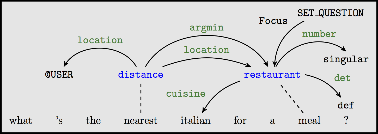
- semantic parsing
- Practical advice
- making things faster
- debugging